


As you build your supply chain model, you will notice slight differences in simulation results between your simulations and the simulations of others who create similar — but not exactly identical — supply chain models.
Small differences in the placement of facilities, the definition of vehicles, and creation of routes add up during the thousands of calculations done by the SCM Globe simulation engine. A facility may run out of products a day or two earlier or later in your simulations than in the simulations of others working on the same case study. Amounts of on-hand inventory and operating costs may differ to some degree. Why does this happen?
Sensitive Dependence on Initial Conditions
As you make changes to the four entities (products, facilities, vehicles, routes), your changes ripple through the model and change the way the model behaves. There are endless changes you can make. And each time you make a change, your simulation takes a trajectory determined by the cumulative effect of all the changes you have made so far. Each person’s simulation results can become increasingly different as they work with their individual supply chain models. Here is why:
In chaos theory, the butterfly effect is the sensitive dependence on initial conditions in which a small change in one state of a deterministic, nonlinear system can result in large differences in a later state. The name of the effect, coined by Edward Lorenz, is derived from the metaphorical example of the details of a hurricane (exact time of formation, and exact path taken) being influenced by minor perturbations such as the flapping of the wings of a distant butterfly several weeks earlier. Lorenz discovered the effect when he observed that runs of his weather model with initial condition data that was rounded in a seemingly inconsequential manner would fail to reproduce the results of runs with the unrounded initial condition data. A very small change in initial conditions had created a significantly different outcome. (Wikipedia: The Free Encyclopedia – “Butterfly effect” – http://en.wikipedia.org/wiki/Butterfly_effect)

Yet regardless of these differences, simulations still show which supply chain designs work best in any given situation. They show whether trucks or railroads or airplanes or ships work best in that situation. They show the best locations for different facilities, and they show how inventory flows through those facilities. They also identify facilities in a supply chain where problems are most likely to occur, and provide useful data for deciding how to respond to those problems.
The Best Solutions are Known as “Attractors”
In the mathematical field of system dynamics, an attractor is a set of numerical values toward which a system tends to evolve from a wide variety of initial starting points. When combinations of system values get close enough to an attractor (an optimal state), the system will remain stable near the attractor, even if small changes are made to individual system values. (Wikipedia: The Free Encyclopedia – http://en.wikipedia.org/wiki/Attractor)
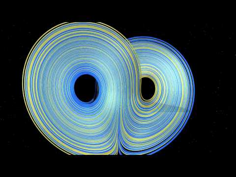
Although each individual simulation follows its own unique trajectory, if you use the simulation results to keep adjusting your supply chain model so as to minimize cost and inventory while always meeting product demand, then your supply chain model, and all other models in a given situation, will converge on one or two best solutions known as “Attractor” solutions as shown in the diagram below.
Imagine the X, Y and Z axes in the diagram are measures of utilization for inventory, transportation and storage in a supply chain. Think of the best solutions as being orbits (blue lines) in the diagram that take the shortest distances to circle around one or the other of the two center circles in the diagram below. As situations change and the relative importance assigned to inventory, transportation, and storage also changes, the position of the optimal center circles will move as well. The shelf-life of optimal answers becomes shorter and shorter as change and unpredictability increases. So supply chains are always adjusting their operations and seeking optimal solutions as they respond to a changing world.

All supply chains operating in a given situation will achieve optimal performance in a similar manner. They will all converge on one or two attractor solutions. An attractor solution for a supply chain model is represented by a combination of entity attributes (values for products, facilities, vehicles, routes) that optimizes overall supply chain performance in a particular situation (read more about this in “Supply Chain Optimization & Reporting Template“).
Once different supply chains get close enough to an attractor solution, small changes or differences in their values for products, facilities, vehicles and routes do not have a significant impact. Despite these small differences, overall performance of these supply chains remains close to optimal for all of them (read more about this in “All Supply Chain Models are Approximations“).
In the real world supply chains can neither attain nor maintain perfect optimization because there are too many unpredictable and uncontrollable variables at work. Real supply chains can approach optimal solutions, but random variances will always force operations to be less than optimal. Supply chains must continuously adjust their operations as situations change. Effective use of people, process and technology enables supply chains to learn and respond so as to get closer and closer to optimal states (attractor states), and stay closer for longer and longer periods of time.
SCM Globe is a Deterministic, Nonlinear System
We are used to working with relatively simple linear models where cause and effect is clear, and where only certain types of changes can be made. SCM Globe is not a simple linear system. It is a virtual sandbox where you can make an unlimited number of changes in any combination you want, and then run simulations to see what happens. It is a deterministic, nonlinear system.
Small changes in one part of an SCM Globe model can produce unexpected or counter-intuitive results in other parts of the model (this happens in the real world too). It can be puzzling, even alarming. And at times it will cause more than a little frustration as you try to figure out how to respond to these results.
You may come to believe your simulation results indicate a bug somewhere in the software (and there may be — no piece of software longer than a few lines of code can ever be proven to be entirely free of bugs). So when in doubt, download the simulation data into a spreadsheet and check the math (be sure to read the answer to Questions 2 and 3 in FAQs). In the downloaded simulation data, pick a facility or a product and track it day by day through the simulation. What do you see?
Most likely you will find that the numbers do add up. But the result is unexpected. There isn’t a bug… but there is a butterfly!
More Insights into the Butterfly Effect and Nonlinear Dynamics
- Quick read and interesting article in Forbes “Chaos Theory, The Butterfly Effect, and the Computer Glitch that Started It All“
- Clear explanation of “strange attractors” and how they were discovered by Edward Lorenz while building his original computer weather model.
- Engaging video by two professors at University of Nottingham, UK. They demonstrate results of the Butterfly Effect in simple systems such as double-jointed pendulums and pool balls traveling across a pool table; and in complex systems such as evolving weather patterns and storms.

[ DISCLAMER: Developers and users of SCM Globe have run thousands of different simulations and analyzed the results thousands of times since release of version 1.0 of the simulation engine in the fall of 2011. In that original version and succeeding versions, bugs were found and fixed, and the accuracy of certain calculations was improved. In this current version (Ver 2.7, in production since October 2013) there are known bugs in editing and displaying supply chain data and they are listed in the FAQs. But no bugs have been found in the actual supply chain simulations, even as usage has increased significantly. If you do find a bug please contact us immediately, and send the simulation data that reflects this bug. Be sure to read the FAQs section to see why deliveries are sometimes missed, and understand the “Day 0” calculations used to start all simulations.]